Tag Archives: Linux

Improving my home Internet performance

For a long time I’ve experimented with shaping my upstream traffic via Linux’s traffic management functionality (tc command) with the goal of improving my Internet connection’s performance. The latest incarnation of this configuration can be found in this script. Anecdotally this configuration greatly improves interactive performance. Use cases such as Skype calls work without a hitch with any other network tasks I want to run at the same time. In this post I provide some simple experimental results and compare against the default configuration.

The goals of the linked tc script are twofold: improve performance under load and stop any single host from monopolizing the available bandwidth. Performance under load is improved by shaping to just below the link bandwidth which stops packets from queuing in the DSL modem and thereby allows the Linux QoS features to manage the traffic. Achieving host fairness is accomplished by hashing the hosts on the network across a set of buckets.  Flow fairness is accomplished via the underlying fq_codel QDisc.

Subset of my home network

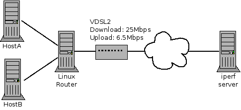
Figure 1: Subset of my home network

Figure 1 shows the layout of the network. Note that when I performed these tests I didn’t disconnect all other devices so these aren’t perfect lab style results.

iperf and ICMP ping

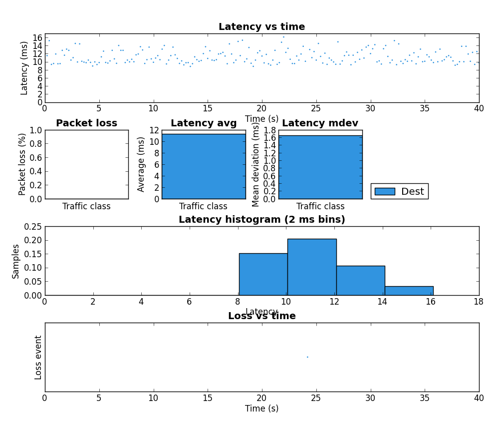
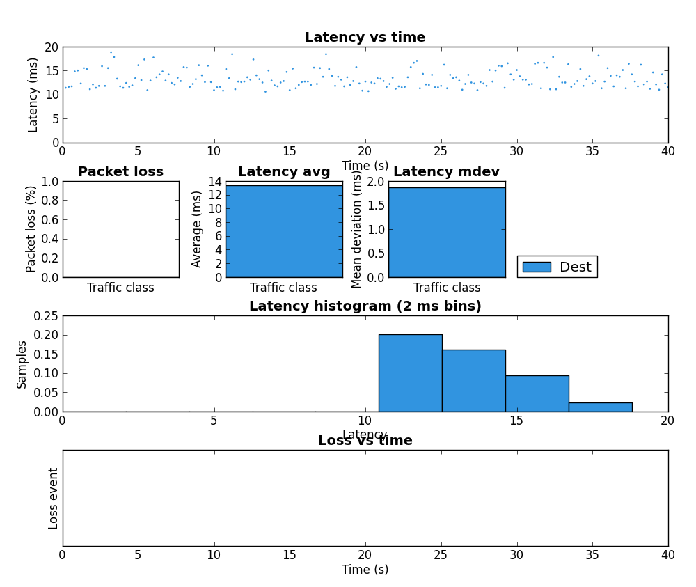
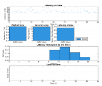
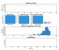
The fist test involves running iperf set to 200kbps and 500 byte packets. This is meant to be somewhat similar to what an interactive application such as a Skype call would produce. The second test used my pingexp utility to chart the ICMP ping results. For both, six different load scenarios were tested (the rows in the table). In both cases the base load was generated from HostA and the test load was generated on HostB.

 Description iperf 200kbps, 500 byte packets (HostB)
ICMP ping results [via pingexp] (HostB)
1 Unloaded 0% loss / 0.229 ms jitter  1
2 Unloaded with tc script 0% loss / 0.197 ms jitter
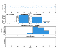
  2
3 Three scp from HostA
0.6% loss / 2.6 ms jitter
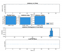
  3
4 Three scp from HostA with tc script 0% loss / 0.496 ms jitter  4
5 iperf 8Mbps, 1400 byte packets from HostA
[Attempted twice, failed on first attempt] 69% loss / 1.58 ms jitter  5
6 iperf 8Mbps, 1400 byte packets from HostA with tc script 0% loss / 0.804 ms jitter 6

Notice the large decrease in latency between rows 3 and 4. This is the result of shaping to below the link rate which stops the buffer in the DSL modem from filling.

The biggest improvement can be seen the last two rows of the table. Without the tc script there is a large amount of packet loss but with the tc script in place HostB’s traffic is affected very little by HostA’s. Due to the use of fq_codel as the underlying QDisc, it is very likely these results would be very similar if both iperf instances were run on HostA but this was not tested.

scp

The third experiment duplicated the six load scenarios above but instead used a single scp transfer on HostB as the test load. Figure 1 shows the result as captured and charted by Wireshark. Each of the six scenarios were run for approximately 20 seconds.

Bitrate of scp from HostB during test scenarios

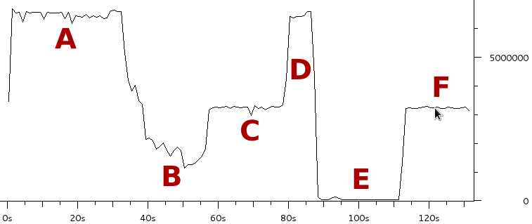
Figure 1: Bitrate of scp from HostB during the six test scenarios

The region marked A corresponds to the two unloaded scenarios (rows 1 and 2 in the table above). As expected there is little difference as both scenarios max the upstream link when there is no contention.

Notice how much the rate drops in region B (row 3 in table) when the three scps are started on HostA. The bitrate is approximately 1/4 of the link rate which is expected since there are four scps running.

Region C (row 4 in the table) has the same four scps but with the tc script in place HostB gets 50% of the link rate and therefore HostA’s three scps share the other 50%. This shows that the tc configuration achieves per host fairness in terms of bandwidth allocation.

Region D should be ignored as it is the result of me taking too long to setup scenario 5.

Region E (row 5) is very interesting. This is where the 8Mbps iperf UDP flood starts. Notice that the scp from HostB is completely drowned out and is effectively unable to transfer any data. This is an extreme example of the kind of dramatic performance drop under load which many have come to expect from busy Internet links. As we’ll see in region F, this is not a fundamental problem with the Internet, it is the result not properly managing the buffers.

Region F (row 6) consists of the same traffic as region E expect the tc script is now in place. Like region C, HostB is now getting 50% of the available bandwidth even though HostA is trying to transmit at a rate higher than the total link rate. This shows that a bit of active queue management can make an Internet connection usable under high load.

Web Traffic

To get a sense for what difference the tc configuration makes to web performance I ran Google Chrome in benchmarking mode for the same six scenarios. The results are presented in the table below.

  url iterations via spdy doc load mean paint mean total load mean stddev Read KBps Write KBps # DOM
1 http://www.google.ca 25 false 186.7 199.7 490 188 NaN NaN 270
2 http://www.google.ca 25 false 176.2 190 380.7 181.4 NaN NaN 270
3 http://www.google.ca 25 false 834.6 843.6 1506.8 1044.6 NaN NaN 270
4 http://www.google.ca 25 false 178.2 192.4 416.7 226.1 NaN NaN 270
5 http://www.google.ca Failed Failed Failed Failed Failed Failed Failed Failed Failed
6 http://www.google.ca 25 false 175.4 188.3 380.5 176.4 NaN NaN 270

I have marked the entries in row 5 as failed because after 120 seconds a single page load had not yet completed.

Like above, the interesting rows to contrast are three and four as well as five and six. In both cases the tc configuration greatly reduced the time required to load www.google.ca.

Summary

This post presented results which showed that the performance and predictability of a DSL residential Internet connection can be greatly improved with some basic traffic management running on a Linux router. If you don’t have a Linux router you may still want to take a look at the configuration of your home router. If it supports bandwidth shaping, try setting it to just below your link rate. The results won’t be as good as presented here but it should make a noticeable improvement.

Making the Linux flow classifier tunnel aware

Flow Classifier

The Linux kernel has many different tools for managing traffic. One of them is the flow classifier which allows the user to configure which fields of the packet headers should be used to create a hash which is then used to identify flows and manage them. For example, if the user selects src,dst,proto,proto-src,proto-dst they get a unique value for each flow (within the limits of the hash). Alternatively, using only src as the key will result in all flows being grouped by the source IP address.

The Problem

Below is a slightly simplified version of my home network.

Figure 1: Simplified home network

All of the traffic, both IPv4 and IPv6, is tunnelled through a Linux router which lives at my service provider. The reason for this complicated setup is that it gives me control of the traffic in both the upstream and downstream. By shaping the traffic to just below the maximum rate in each direction I am able to avoid Bufferbloat problems and prioritize latency sensitive traffic such as SSH, DNS and Vonage. Especially under load, my QoS scripts make marked difference in how fast the Internet feels.

The multiple tunnels present a problem for implementing my QoS scheme because from the perspective of the underlying interface there are only two flows on the network. One for the IP-IP tunnel and one for the IP-IPv6 tunnel. A work around I used for a while was to apply the QoS rules to the IP-IP tunnel interface because that’s where the bulk of the traffic flows. However, this meant that IPv6 traffic was not properly controlled and any time I had a significant amount of IPv6 traffic I lost all the advantages of my QoS scheme.

To solve this properly I needed a way to look into the tunnels in order to identify the inner network flows. So I’ve extended the flow classifier with the keys in the following table. IP-IP, IP-IPv6, IPv6-IP and IPv6-IPv6 tunnels are supported.

Key Description
tunnel-src Extract the source IP from the inner header
tunnel-dst Extract the destination IP from the inner header
tunnel-proto Extract the protocol from the inner header
tunnel-proto-src Extract the transport protocol source port from the inner header
tunnel-proto-dst Extract the transport protocol destination port from the inner header

 Results

In order to validate that this works I started a couple SCP uploads to max the upstream bandwidth and then ran ping-exp to measure the latency. At the start of the test the flow classifier keys were src,dst,proto,proto-src,proto-dst. Approximately half way through I changed the keys to src,dst,proto,proto-src,proto-dst,tunnel-src,tunnel-dst,tunnel-proto,tunnel-proto-src,tunnel-proto-dst. The advantage of keeping the non-tunnel keys is that any traffic created by the router itself is still classified properly. Here is the tc script I used. You can see the results of this test in the figure 2 below.

Figure 2: Before and after tunnel keys

For the first half of the test you can see the high latency. This is due to all the traffic from the SCP upload and ICMP pings being placed into the same queue because from the perspective of the flow classifier there is only one flow. In the second half of the test the addition of the tunnel keys allows the flow classifier to place the ICMP packets into a different queue which is not affected by the SCP upload and therefore has much lower latency. The large amount of packet loss during the key change is because the script I used creates a large number of queues. While these queues are being created packets are dropped.

While my network setup may be a bit unique I think it’s likely that many home networks will have some form of tunnelling in the near future as tunnels are part of several IPv6 migration strategies. So hopefully this little addition will be useful in many different contexts.

Below are links to the two patches that are required. I’ll post them to Netdev for review shortly.

clsflow-tunnel-20111016.patch

iproute-clsflow-tunnel-20111016.patch

Linux flow classifier proto-dst and TOS

Recently I’ve been playing around with the Linux flow classifier on my gateway. The flow classifier provides the ability to group network flows by configuring which parts of the packet headers (referred to as keys) are used in a hash calculation which chooses the output queue.

All of my Internet traffic travels over an IPIP tunnel to another Linux box. I do this so I have control of the QoS in both the upstream and the downstream. A result of this configuration is that from the perspective of the output interface there is only a single network flow.

I configured the flow classifier to use the src,dst,proto,proto-src,proto-dst keys which aims to provide 5-tuple flow fairness. Here’s the simple tc script I used. Due to the IPIP tunnel I expected to see that all traffic would be placed into the same queue. Strangely, the below is what my little ping-exp utility showed when running at the same time as an SCP upload.

Figure 1: Unexpected flow classifier behaviour

Coincidentally I ran ping-exp configured to send three different streams of ICMP traffic with different IP TOS values. Note that SCP automatically sets the IP TOS to the equivalent of the “Low” stream in the test.

Notice that the pings using the high and default TOS values appear to be unaffected by low priority ping and SCP traffic. This was unexpected because none of src,dst,proto,proto-src or proto-dst keys should be affected by the TOS value.

After a bit of experimentation I determined that the proto-dst key was the source of the problem. If you spend a bit of time with the flow_get_proto_dst() function in cls_flow.c you’ll see that if the protocol is ICMP or IPIP, as it is in my test, then the following value is returned:

return addr_fold(skb_dst(skb)) ^ (__force u16)skb->protocol;

skb_dst() returns a pointer to a dst_entry structure. Since Linux maintains separate dst_entry structures for each destination,TOS pair the source of the unexpected behaviour is obvious.

I’m not knowledgeable enough about the Linux network stack to be certain but I don’t see any value in returning a value for proto-dst which is random with respect to the actual traffic on the wire. At the very least this is not intuitive behaviour.

If you look at flow_get_proto_src() you’ll see something similar:

return addr_fold(skb->sk);

In this case a pointer to the local socket structure is used as a fallback. Again, this has no relation to the actual packets on the wire and if the packet does not originate at the local machine then no socket exists which causes this value to be zero anyway.

It seems to me that the most intuitive behaviour would be to have the proto-src and proto-dst keys return zero when they are applied to traffic that doesn’t have the notion of transport layer ports.

I’ll post to Netdev about this and see what the kernel devs have to say.

Related to this, I have a patch to the flow classifier that adds tunnel awareness which I plan post to Netdev this weekend as well.

pfifo_fast and ECN

Summary

The default queuing discipline used on Linux network interfaces deprioritizes ECN enabled flows because it uses a deprecated definition of the IP TOS byte.

The problem

By default Linux attaches a pfifo_fast queuing discipline (QDisc) to each network interface. The pfifo_fast QDisc has three internal classes (also known as bands) numbered zero to two which are serviced in priority order. That is, any packets in class zero are sent before servicing class one, any packets in class one are sent before servicing class two. Packets are selected for each class based on the TOS value in the IP header.

The TOS byte in the IP header has an interesting history having been redefined several times. Pfifo_fast is based on the RFC 1349 definition.

   0     1     2     3     4     5     6     7
+-----+-----+-----+-----+-----+-----+-----+-----+
|   PRECEDENCE    |       TOS             | MBZ |  RFC 1349 (July 1992)
+-----+-----+-----+-----+-----+-----+-----+-----+

Note that in the above definition there is a TOS field within the TOS byte.

Each bit in the TOS field indicates a particular QoS parameter to optimize for.

Value Meaning
1000 Minimize delay (md)
0100 Maximize throughput (mt)
0010 Maximize reliability (mr)
0001 Minimize monetary cost (mmc)

Pfifo_fast uses the TOS bits to map packets into the priority classes using the following table. The general idea is to map high priority packets into class 0, normal traffic into class 1, and low priority traffic into class 2.

IP TOS field value Class
0000 1
0001 2
0010 1
0011 1
0100 2
0101 2
0110 2
0111 2
1000 0
1001 0
1010 0
1011 0
1100 1
1101 1
1110 1
1111 1

This approach looks reasonable except that RFC 1349 has been deprecated by RFC 2474 which changes the definition of the TOS byte.

   0     1     2     3     4     5     6     7
+-----+-----+-----+-----+-----+-----+-----+-----+
|               DSCP                |    CU     |  RFC 2474 (October 1998) and
+-----+-----+-----+-----+-----+-----+-----+-----+    RFC 2780 (March 2000)

In this more recent definition, the first six bits of the TOS byte are used for the Diffserv codepoint (DSCP) and the last two bits are reserved for use by explicit congestion notification (ECN). ECN allows routers along a packet’s path to signal that they are nearing congestion. This information allows the sender to slow the transmit rate without requiring a lost packet as a congestion signal. The meanings of the ECN codepoints are outlined below.

   6     7
+-----+-----+
|  0     0  |  Non-ECN capable transport
+-----+-----+

   6     7
+-----+-----+
|  1     0  |  ECN capable transport - ECT(1)
+-----+-----+

   6     7
+-----+-----+
|  0     1  |  ECN capable transport - ECT(0)
+-----+-----+

   6     7
+-----+-----+
|  1     1  |  Congestion encountered
+-----+-----+

[Yes, the middle two codepoints have the same meaning. See RFC 3168 for more information.]

When ECN is enabled, Linux sets the ECN codepoint to ECT(1) or 10 which indicates to routers on the path that ECN is supported.

Since most applications do not modify the TOS/DSCP value, the default of zero is by far the most commonly used. A zero value for the DSCP field combined with ECT(1) results in the IP TOS byte being set to 00000010.

Looking pfifo_fast’s TOS field to class mapping table (above), we can see that that a TOS field value of 00000010 results in ECN enabled packets being placed into the lowest priority (2) class. However, packets which do not use ECN, those with TOS byte 00000000, are placed into the normal priority class (1). The result is that ECN enabled packets with the default DSCP value are unduly deprioritized relative to non-ECN enabled packets.

The rest of the mappings in the pfifo_fast table effectively ignore the MMC bit so this problem is only present when the DSCP/TOS field is set to the default value (zero).

This problem could be fixed by either changing pfifo_fasts’ default priority to class mapping in sch_generic.c or changing the ip_tos2prio lookup table in route.c.

Linux x86_64 and Javascript

The competition between browsers in the area of Javascript performance has led to some pretty dramatic performance increases in the last couple of years. A lot of this has been accomplished through Javascript just in time (JIT) compilers. What JITs do is convert the Javascript into native instructions which execute a lot faster than more abstract forms. The one downside to this approach is that each native architecture must be supported to get the speed boost.

If you follow Javascript performance you know that recent versions of Firefox have a JIT. What you may not know is that there is no JIT in Firefox for x86_64. This isn’t that big of a problem for Windows since there are so few 64-bit windows users but Linux distributions have been native 64-bit for quite some time. So if you’ve installed a 64-bit version of your faviourite Linux distribution you are getting far slower Javascript performance in Firefox than if you had installed the i686 version. How much slower?

The following benchmarks were executed on an i7-930 running Fedora 12, Firefox 3.5.8 and Epiphany 2.28.2. The benchmarks I used are the SunSpider and V8 Javascript benchmarks.

Browser/arch V8 (higher is better) SunSpider (lower is better)
Firefox i686 PAE 402 1002.6ms
Firefox x86_64 277 2131.2ms
Epiphany x86_64 887 1261.0ms

These results show that the Javascript performance of i686 Firefox is a lot better than x86_64. The Epiphany web browser is based on Webkit which, based on these results, I’m guessing does have a x86_64 JIT.

Linux SFQ experimentation

I’ve been doing some more experimentation with Linux QoS configurations using my ping-exp utility. Today I noticed that whenever I add a SFQ to the configuration there are large latency spikes. After a bit of digging it appears that these spikes happen when the SFQ changes its flow hash. This occurs every perturb interval as configured when the SFQ is created.

Below are the results from a couple experiments which show this behavior. For both experiments I had two outbound ping floods of MTU sized packets. This saturated the outbound link. The experiment itself pinged three other hosts. I made sure to use four distinct hosts (one for flood, three for the experiment) to avoid collisions in the SFQs flow hash.

The PNGs below are not ideal for detailed inspection of the graphs. However, you can also download the data files from the experiment and load them using ping-exp. This allows zooming in on the graph. See the links at the end.

HTB SFQ limit 10 perturb 5

HTB SFQ limit 10 perturb 5

The above graph is based on an experiment where the perturb value was set to five seconds. Although the large latency spikes do not occur at every five second interval, when they do occur they are on the five second grid.

HTB SFQ limit 10 perturb 20

HTB SFQ limit 10 perturb 20

The second experiment used a perturb time of twenty seconds. Again, the latency spikes do not occur every twenty seconds but they do occur on the twenty second grid.

During the experiment I ran a packet capture to make sure there wasn’t any activity that might skew the results. The amount of captured traffic was very small.

The network I performed this experiment on consists of a P3-450 Linux gateway where the QoS configuration is applied to the ppp0 device. The kernel version is 2.6.27.24-170.2.68.fc10.i686. A host behind the gateway was used to generate the ping floods and run ping-exp.

Configuration and data files

HTB SFQ limit 10 perturb 5 script

HTB SFQ limit 10 perturb 5 ping-exp data file

HTB SFQ limit 10 perturb 20 script

HTB SFQ limit 10 perturb 20 ping-exp data file

ping-exp: Ping experiment utility

Recently I’ve been playing with Linux’s QoS features in order to make my home Internet service a little better. Since I’m primarily interested in latency I used ping to benchmark the various configurations. This works reasonably well but it quickly becomes hard to compare the results.

So I decided to build a tool to perform several ping experiments, store the results and graph them. The result of this work is ping-exp.

At present ping-exp can vary the destination host name as well as the TOS field. The interval between pings and total number of pings is globally configurable. The results can be written to a file to be loaded later, output to a PNG or both. Line and scatter plots are supported. When not writing the image to a file ping-exp displays the graph using Matplotlib’s default graph viewer. This allows zooming in on interesting parts of the graph. In the future I’d like to add the ability to specify the ping packet size.

As an aside, Python and Matplotlib make this kind of stuff so much fun.

Below are a few graphs created by ping-exp.

ping-exp example #1

ping-exp example #1

ping-exp example #2

ping-exp example #2

ping-exp example #3

ping-exp example #3